.jpg)
We all know how to learn a new video game: we just play. The first time we play, we lose the game very quickly. And we continue to lose regularly. But with each new game we play, we learn something new that will eventually help us win. Let's be fair: we also learn from experience how to use our brand-new TV, or mobile phone: no one ever reads the manual (unless we can’t figure out a specific functionality). One may wonder if a similar approach can be designed for software systems. And here is where Reinforcement Learning makes its entrance.
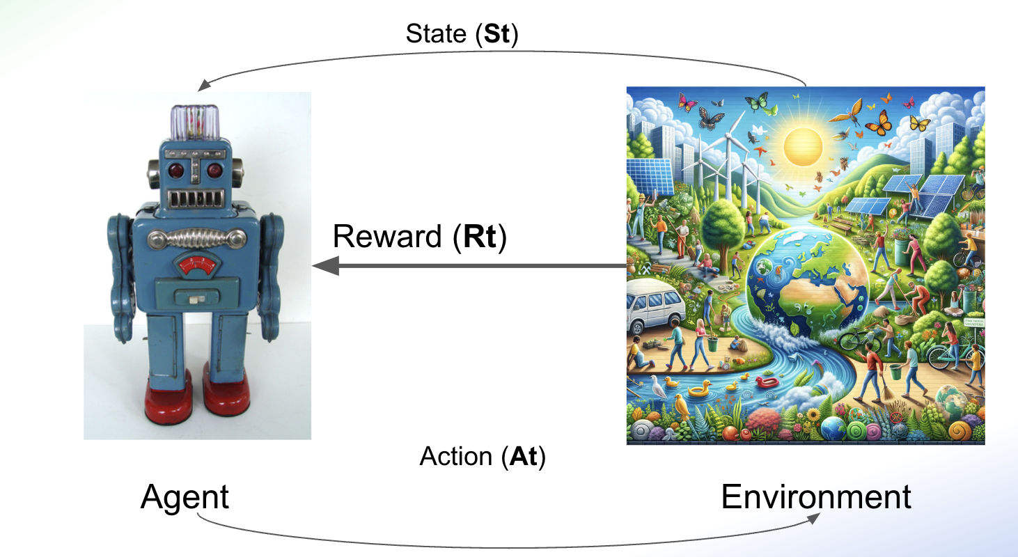
Reinforcement Learning is an AI general framework, where the learning process is done through interaction with the environment. Formally, reinforcement learning is the process by which a software agent interacts with the environment, making observations and taking actions. Each time an action is performed, the agent receives a reward from the environment. In our example of the video game, we (the players) are the agents; the environment is the game, each movement we make with the command is the action, the observations are what we see happening on the screen, and the reward is the points we get.
In summary, Reinforcement Learning allows agents to learn optimal strategies by interacting with their environment and adjusting their actions to maximize long-term rewards. The ultimate goal of RL is to develop a versatile algorithm capable of solving a wide array of tasks.
How does it work?
Reinforcement learning's general framework is quite easy to describe: an agent decides the next action by considering the observations and rewards obtained from the environment with the previous actions. The function to decide the next action given the observations and rewards is known as policy and is usually noted with the Greek letter \Pi.
In the book Hands-On Machine Learning with Scikit-Learn Keras and TensorFlow (which I strongly recommend), Aurélien Géron illustrates what a policy strategy is with a very simple example: a robotic vacuum cleaner. Suppose that the objective is to maximize the amount of dust it can take in 30 minutes. The policy could be: at each second, decide between moving forward, rotating to the left or rotating to the right. This policy has only two parameters: whether to move forward or rotate, and then the rotation angle. The question is: how can we learn what are the best parameters to maximize the amount of dust that the cleaner picks up ? Deciding what is the best option is not trivial: is it better to do it sequentially (for instance: first move forward, next rotate to left and next rotate to right) or maybe a completely random process is preferred ? One possibility is to try different combinations of each parameter. The problem is that this approach does not scale to real problems. In fact, even in the case of the vacuum cleaner which only has two parameters, the number of combinations grows exponentially at each time step. Even if we simplify at the extreme the problem of having just three possible actions: move forward, rotate right or rotate left (we are not considering for instance the angle of rotation), in 10 seconds we have nearly 60000 possibilities, and just in a minute the number reaches the incredible number of 4.2e28 ! Clearly, we cannot use brute force to analyze all possible values. This is one of several challenges that we will face when dealing with RL problems. Let's take a deeper look at those challenges and different options to deal with them.
Challenges in implementing Reinforcement Learning
Let's illustrate the difficulties of implementing RL algorithms with another example, this time from another excellent book, “Understanding Deep Learning” by Simon J.D. Prince.
Consider learning to play chess. At the end of the game, a given player has three possibilities: win, lose, or draw. Based on these outputs, we can define a reward function as follows: we give a +1 if the player wins, a -1 if the player loses, and 0 if it is a draw and also for any other intermediate step (because while playing, nobody wins or loses).
This simple example illustrates several of the problems that we face when implementing RL algorithms:
- The reward can be sparse. For example, in this case, it is limited to only three possible values, and they are only known at the very end of the game.
- The reward is temporally offset from the action that causes it (for instance, moving the tower in the middle of the match). The problem is that to understand the value of each action at any state, we need to associate the reward with this action. This problem is termed the credit assignment problem.
- The environment is not deterministic: the opponent doesn’t always make the same move in the same situation, so it’s hard to know if an action was truly good or just lucky.
- Finally, the agent must balance exploring the environment (e.g., trying new opening moves) with exploiting what it already knows (e.g., sticking to a previously successful opening). This is termed the exploration-exploitation trade-off.
Let's see how these challenges can be tackled with different algorithms and techniques.
Key elements of reinforcement learning
The credit assignment problem
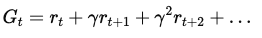
We have seen that in most cases, the reward is not linked to the immediate action. Thus, taking the action that maximizes the reward is not easy because, as we've seen in the previous example, the reward may be far in the future (and the action has to be taken now). One of the ways to deal with this problem (known as the credit assignment problem) is to evaluate an action based on the sum of all the rewards that came after it. Usually, the rewards are not summed directly but after applying a discount factor $\gamma$. The sum of all rewards with the corresponding discount for a given action is called the return of the action:
Because one action will be followed by other actions that are not always the same (for instance, given the exact same state of the game, the opponent may take a different action), only one run will not be enough to learn the good actions. The process then is to play several times (or if it is a virtual environment, run several times the environment), keep track of all action returns, compute the mean and standard deviation and normalize the action returns. This will give us an idea of how good or bad an action is on average. This is called the action advantage. This idea of computing the reward taking into consideration future rewards is applied in most of the algorithms and methods that we will be analyzing in the next sections.
Exploration vs Exploitation
During the learning process, as the agent plays the game or runs the simulation, it must balance two strategies: taking random actions to explore the environment (exploration) or choosing actions that maximize the known expected return based on current information (exploitation). Gerón illustrates this dilemma with an analogy: imagine you have a favorite restaurant where you once tried a dish that left an unforgettable impression. While you know you love that dish, and most of the time you choose this option from the menu, exploring other menu options might lead to an even better discovery. So if you never try something different, you may be losing the opportunity to increase your reward.
One way to deal with this dilemma is to add some randomness to the action selection policy. For instance, we can decide to take the action that maximizes most of the time but in a few of them, we just take a random action. Here is a python pseudo-code of such a policy:
def policy(state, epsilon):
if np.random.rand() < epsilon:
return random_sample(possible_actions)
else:
best_action = model.predict(state)
return best_action
Markov Decision Process
Markov Decision Processes have been presented by Richard Bellman in 1957 as a way of modeling RL problems. Markov Decision Process is derived from Markov Chains. In a Markov Chain, we have several states and on each state we have the probability to move to the next one. Here is a classical example of a Markov Chain:
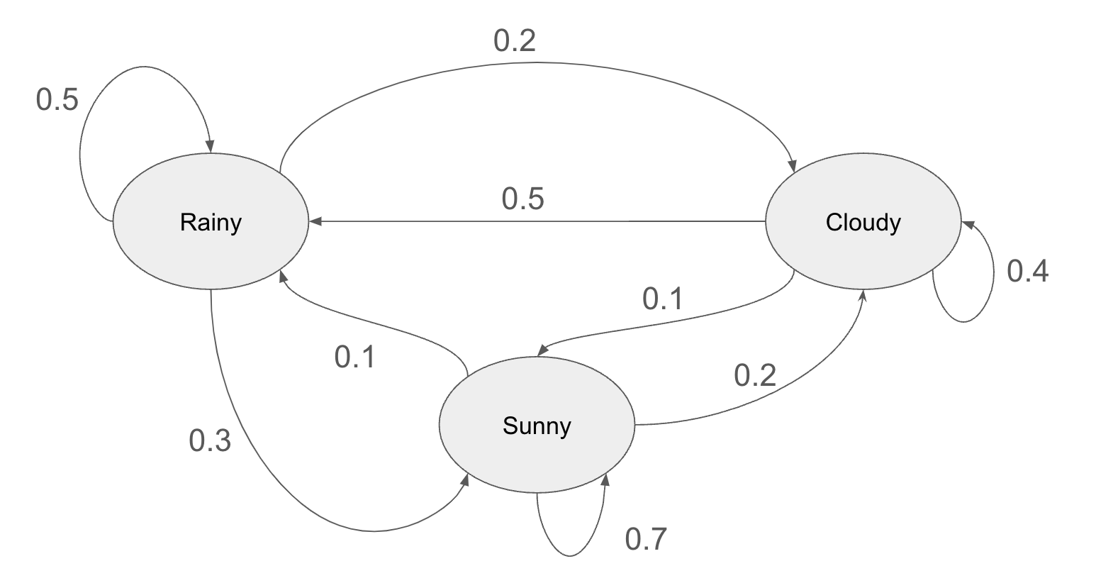
For each possible state (rainy, sunny or cloudy), there is a probability to move to any other state (and even stay in the same state). One important property of the Markov Chains is that the probabilities to move to a new state only depends on the actual state and not on the history of the states. In this example, it doesn't matter if it's raining for 10 days: the probability of moving to another state is exactly the same as if it was raining for 10 minutes.
Markov Decision Process incorporates two additional components to the Markov Chains. First of all, in each state the agent can take a number of actions, and each one of these actions has a different probability of ending up in a new state. Secondly, some of these actions have rewards. In the article Markov chains and Markov Decision process, the authors present this nice example.
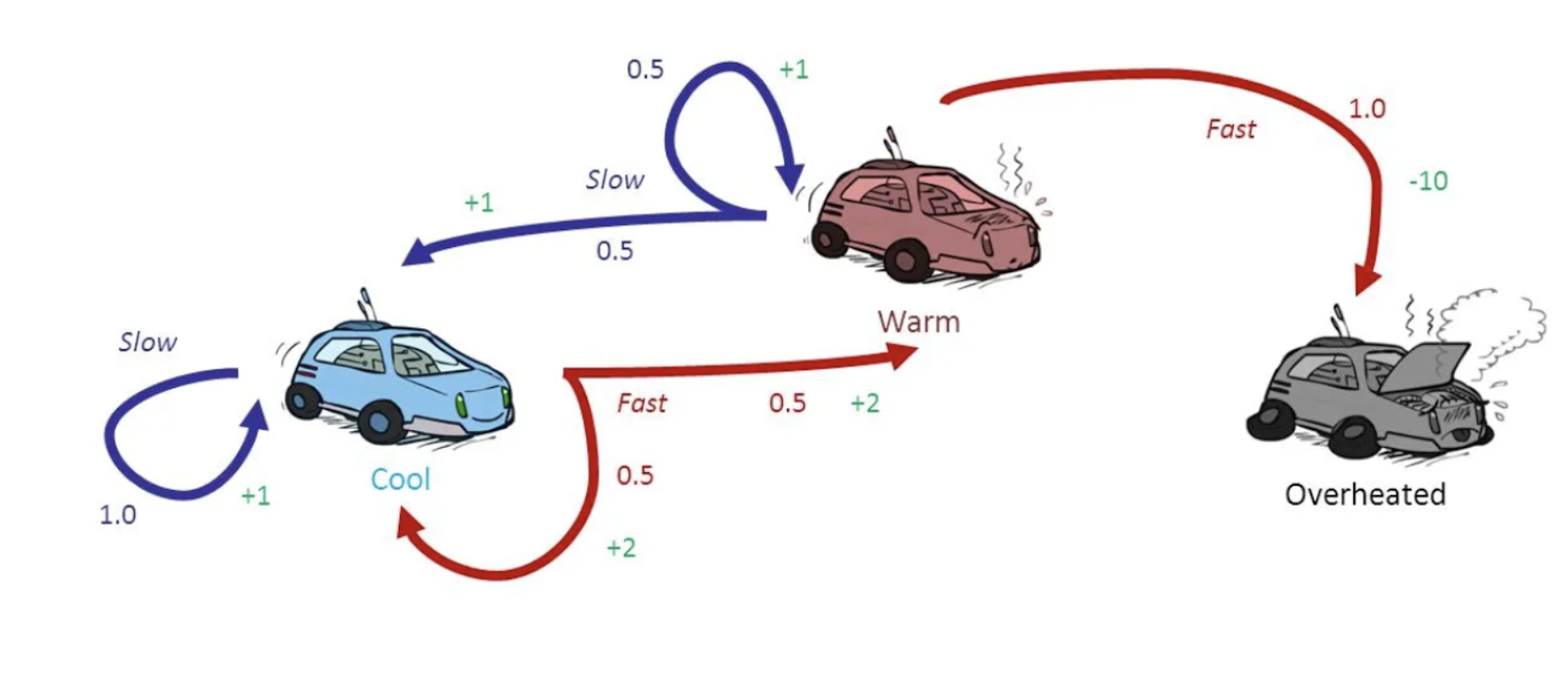
Suppose that we have a game in which the idea is to obtain the maximum reward in a fixed time. In this game, the car has three possible states: the engine is either cool, warm or overheated. The possible actions that the car has are two: slow down or go faster. The caveat is that if the car reaches the “overheated” state, the process ends and a penalty is applied to the obtained reward so far.
The idea behind modeling a RL problem as a Markov Decision Process is to analyze the environment in order to define a policy that maximizes the reward. If we just think of the immediate reward, the problem is simple: given a state s (for example, cool), let's take a look at the two possible actions: go slower or go faster. If we decide to slow down, we have only one state, which is to keep cool and the reward that we obtain is +1. If we decide to go fast then two states are possible with the same probability: either stay cool or warm. In each case, the reward is +2. If we just take a look at the next step, then the best option seems to be to go faster: in any case we will obtain a reward of 2, while if we go slower then the reward will always be 1. But this approach is not taking into consideration the “future” reward that we may obtain after one decision: we need to also consider the value of each one of these new states.
This led us to the Bellman equation:
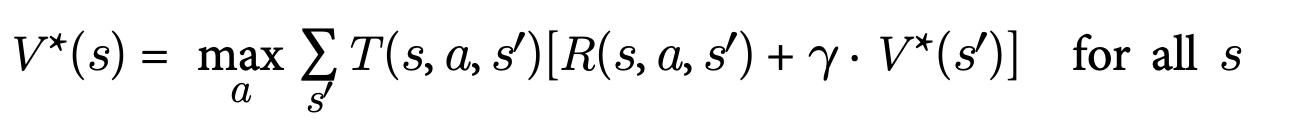
Bellman showed that if the agent acts optimally, the optimal state value is the sum of all discounted future rewards the agent can expect on average after it reaches the state. In other words, given a state s, the best action an agent can take is the one that on average maximizes the reward with the discount.
From this equation, we can derive an iterative process that approximates the solution:
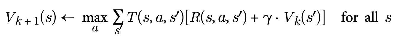
Q-Value Iteration Algorithm
Knowing the optimal state values can be helpful, especially for assessing a policy, but it does not directly provide the agent with the best policy to follow. Fortunately, Bellman introduced a similar method to estimate optimal state-action values, commonly referred to as Q-values (quality values). A Q-Value represents the expected cumulative reward from a state-action pair (s,a), assuming the agent follows an optimal policy afterward.
The optimal Q-value for a state-action pair (s,a), denoted as Q∗(s,a), represents the total discounted future rewards the agent can expect on average after reaching state s, taking action a, and then acting optimally for all subsequent steps. This estimation is made before observing the result of the chosen action.
Given the optimal Q-Values, the policy is very simple: for a state s, choose the action that maximizes Q:
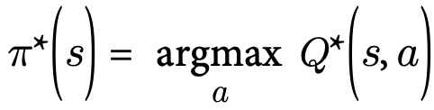
This algorithm is known as the Q-Value iteration algorithm.
Temporal Differential Learning
The process explained so far assumes that we have a complete knowledge of the environment: we know all the transition probabilities between states and we also know the rewards. In most situations, this is not the case. For instance, we need to play several times on a flight simulator before knowing how to press the keys to have a peaceful landing. In most situations, the probabilities of the states and the rewards are learnt as we play. The Temporal Differential Learning algorithm is very similar to the Q-Value algorithm presented before but with a modification that takes into account that the agent has no knowledge of the environment and that both the probabilities transitions and the rewards have to be learnt. For that, the agent uses an exploration policy, and as it plays the game or navigates through the virtual environment, it estimates the state values based on the rewards and the transitions observed:

We can see that this algorithm performs an average between the previous value Vk(s) and the reward with the discount if the new state is s’. Because we need to revisit this several times, different s’ will be considered and all of them will be summed to the Vk(s). The parameter alpha, known as the learning rate, controls the amount of information added at each step.
Q-Learning
When the exploration technique is applied to the Q-Values, we end up with another algorithm called Q-Learning. Here again, Q-Values are learnt as the agent plays or interacts with the environment:
Q(s,a){k+1} = (1-alpha) Q(s,a)k + alpha(r + \gamma \max_a’ Q(s’,a’))
For each state-action pair (s,a), the algorithm maintains a running average of the rewards r the agent receives after choosing action a in state s. Additionally, it updates this average with the discounted sum of expected future rewards. To estimate this sum, the algorithm uses the maximum Q-value of the next state s′, assuming the agent will follow an optimal policy from that point onward. This approach ensures the agent progressively improves its policy by leveraging both immediate and future reward signals.
The Q-Learning algorithm is called an off-policy algorithm because the policy being trained can be different from the one used during training. In fact, given enough iterations, purely random exploration policies can achieve very good results.
Deep Reinforcement Learning
Any of the aforementioned algorithms have a problem when facing real world problems: they do not scale. Even for the most simple games or environments, the number of states is overwhelming. Geron gives the example of the Pacman game: in there, the number of pellets that the Pacman can eat are 150, which can be present or not. This gives us (2^150 which is nearly 10^45). And this is only considering the pellets: if we have to consider the position and presence of ghosts or Ms. Pacman then the number of possible states is greater than the number of atoms in our planet !
One solution to this problem is to approximate Q(s,a) with a function that depends on a learnable parameter \theta: Q_\theta (s,a). This process is called approximate Q-Learning. And if we use as the family of parametric functions deep neural networks, the process is known as Deep-Q-Learning and the type of networks are called Deep Q-Network (DQN).
How do we train a DQN? Let’s focus on the approximate Q-value predicted by the DQN for a given state-action pair (s,a). According to Bellman's principles, this Q-value should align closely with the actual observed reward r obtained after taking action a in state s, plus the discounted value of acting optimally from the subsequent state s′.
To estimate this future value, we can evaluate the DQN for state s′ across all possible actions a′. This provides approximate Q-values for each action. Assuming the agent will follow an optimal policy, we select the highest Q-value among these and apply the discount factor. This gives an estimate of the sum of discounted future rewards. By adding the immediate reward r to this discounted future value, we compute a target Q-value y(s,a) for the pair (s,a).
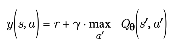
Using the target Q-value, we perform a training step with a gradient descent algorithm. The goal is typically to minimize the squared error between the predicted Q-value, Qθ(s,a), and the target Q-value, y(s,a). Alternatively, the Huber loss can be used to make the algorithm less sensitive to large errors.
Real world examples
Gaming
Obviously, the most well known example of the use of Reinforcement Learning is AlphaGo Zero, a system developed by DeepMind that was able to outperform the version of Alpha Go known as Master that has defeated world number one Ke Jie. Initially, AlphaGo Zero had no prior knowledge of Go, apart from the rules. Unlike previous versions of AlphaGo, Zero did not rely on hand-programmed scenarios to recognize unusual board states; instead, it focused on the board's stones alone. Through reinforcement learning, AlphaGo Zero played against itself, gradually learning to predict its own moves and their consequences on the game. In its first three days, AlphaGo Zero played 4.9 million self-games, rapidly developing the necessary skills to defeat top human players.
Industry automation
Most modern industries have several states in which the production environment can be. For each state, several different actions can be taken, for example, to maintain the quality of the product under certain conditions or to reduce production costs. Thus, reinforcement learning can be a powerful tool to analyze how different actions affect the reward (product quality, production costs, etc.). Given a certain state in which our production environment is, having a RL algorithm that indicates the best actions to take can improve the entire process. An example of this is the cooling strategy developed by DeepMind for Google data centers:
Every five minutes, our cloud-based AI pulls a snapshot of the data centre cooling system from thousands of sensors and feeds it into our deep neural networks, which predict how different combinations of potential actions will affect future energy consumption. The AI system then identifies which actions will minimize energy consumption while satisfying a robust set of safety constraints. Those actions are sent back to the data center, where the local control system verifies the actions and then implements them.
The magic ingredient behind chatGPT: Reinforcement Learning From Human Feedback
If you have ever tried to evaluate a Large Language Model (LLM) on how “good” a piece of generated text is, you will understand the difficulties of formalizing this process. If the text is clearer, or the language is more appropriate for the situation (just to mention a few), all these are difficult parameters to incorporate into an evaluation protocol. But given two models we want to evaluate, we can ask a human what is the one that is preferred for the situation without the need to define explicit rules. Indeed, this is the strategy openai has followed to improve chatGPT (and in fact is still doing: from time to time, two different answers are generated, and you have to tell chatGPT the preferred one). This information is incorporated into a Reinforcement Learning algorithm, where the human basically gives the reward. This type of process is known as Reinforcement Learning from Human Feedback (RLHF). A clear explanation of how this process is implemented for the case of chatGPT is given in OpenAI webpage, where the following image was extracted:
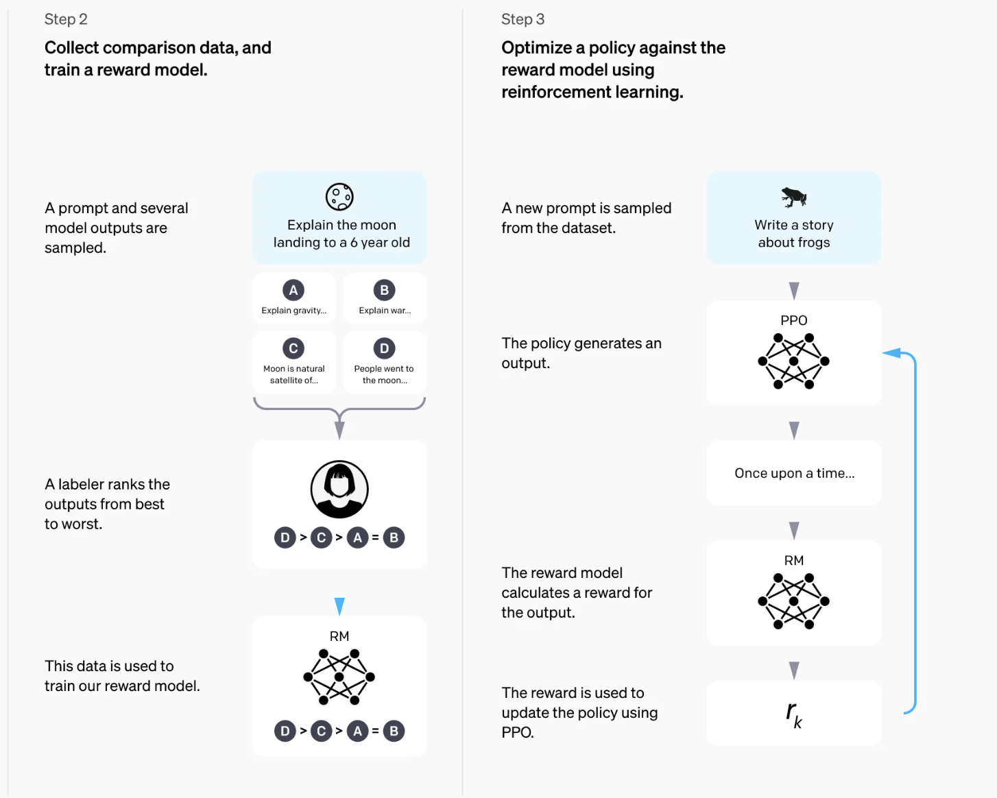
Let's assume that we have several models (A, B, C, D that generate different outputs for the same request (in this case, “Explain the moon landing to a 6-year-old”). The labeler (a human) ranks the models based on which returns a better answer. That information is then used to train a reward model. The second step is incrementally improving the language model using the reward it obtains for different prompts. In this way, the language model is aligned with the rules learned in the reward model (which was trained by the outputs of humans).
Conclusion
Reinforcement learning stands as one of the most relevant fields in artificial intelligence. It presents a general framework that allows agents to learn through trial and error by interacting with their environments. From mastering games like chess and Go to optimizing logistics and resource management in the real world, the applications of reinforcement learning continue to grow. Also robotics and autonomous systems are generally based on reinforcement learning techniques.
Its potential, however, comes with challenges: the computational cost and time required to navigate through the event space creates issues for stability and scalability of learning systems. Nevertheless, innovations such as deep reinforcement learning and advancements in model-based methods are addressing these hurdles, making RL increasingly viable for complex, real-world problems.
As we look ahead, collaboration between academia, industry, and policymakers will be essential to harness RL’s power responsibly, ensuring its use promotes societal and environmental well-being.

.jpg)
.jpg)
.jpg)