.jpg)
Introduction
We are setting large language models and autonomous agents aside, which currently dominate the conversation around AI, and focus today on time series forecasting, a topic that remains a relevant task in industries like energy, retail, and finance. Forecasting research has evolved significantly in recent years, moving from simple statistical methods to complex deep-learning architectures that were pre-trained on several different datasets.
As we explored in our previous article, "Time Series Data: Analysis vs Forecasting Explained" [1], the goal of forecasting is to leverage historical patterns to predict future values. Achieving high accuracy in production involves more than just looking at past data; it requires understanding how different model architectures work under the hood and when it makes sense to choose a newer, more complex model instead of a proven legacy architecture.
In this article, we will provide an overview of the current state of the art, categorizing models into distinct "families" and discussing how to select the right tool for your specific use case.
Data: Beyond Historical Values
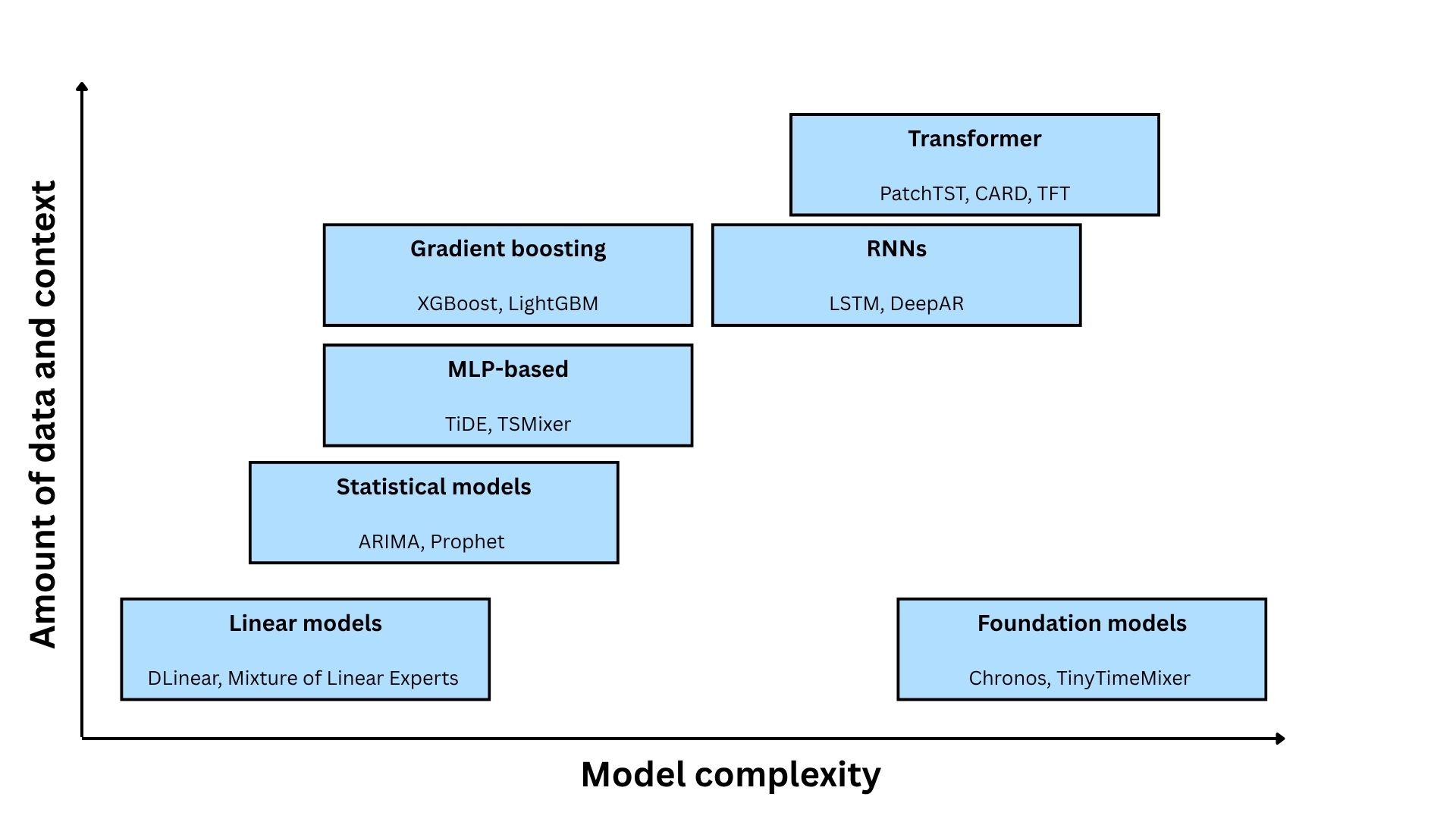
While the model itself is the centerpiece of the forecasting system, data is the primary driver of predictive performance. Even the most sophisticated transformer will fail if the input data is insufficient or poorly conditioned. As illustrated above, data quality and quantity is crucial when selecting a model architecture. While a simple linear model can generalize well with limited history, deep learning architectures are data-hungry. Without enough "contextual diversity", meaning enough examples of how different covariates interact, complex models are prone to overfitting, essentially memorizing noise rather than learning the underlying signal.
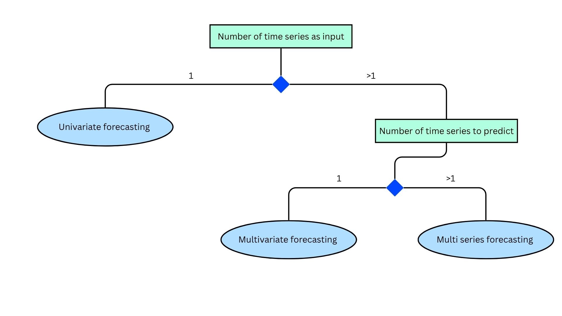
In addition to the target variables, i. e. the historical values of what you are trying to predict, it is also useful to consider the surrounding context. Forecasting tasks can be split into different categories depending on the available data.
- Univariate forecasting: Only the historic values of the target variable are available for the predictions.
- Multivariate forecasting: In addition to the target variable, other relevant sources of information (i.e. covariates) are present. These can either be other time series (dynamic covariates) from past observations or future known values, or time invariant data (static covariates).
- Multi-series forecasting: The model should predict multiple time series that are correlated.
With these preliminaries described, let’s take a closer look at the different model families, their inner workings and when they would be an appropriate model choice.
The Baseline: Statistical Foundations
Statistical models are a very viable starting point for most forecasting problems, given that they are fast to train and interpretable by design.
ARIMA [2] (Auto-Regressive Integrated Moving Average) combines three components. The autoregressive (AR) part expresses the current value as a weighted combination of past values. The integrated (I) part applies differencing to remove non-stationarity. The moving average (MA) part corrects predictions using lagged forecast errors. This model has decent performance on stationary univariate series with little data, but struggles with multiple seasonalities and data with structural breaks. Some further variations were built on top: SARIMA, which adds a seasonal component and SARIMAX, which also includes covariates.
Prophet [3], developed at Meta, decomposes the time series into trend, seasonality, and holiday effects. Seasonality is modeled via Fourier series, the trend is piecewise linear or logistic with automatic changepoint detection. This model also has the capability of forecasting confidence intervals through probabilistic modelling.. Prophet specifically models special dates such as holidays, capturing their potentially irregular timing and localized impact through user-defined event regressors. It thrives when the dominant signal is composed of trend and multi-period seasonality.
Classical machine learning: Gradient boosting
When your data includes rich feature sets, mixed data types, and relatively modest sequence lengths, gradient boosting methods remain a very suitable option for forecasting. Some of the most popular ones are LightGBM [4] and XGBoost [5]. Gradient boosting is an ensemble learning technique that builds a sequence of weak predictive models (typically decision trees), where each successive model is trained to correct the residual errors left by the previous ones, progressively improving overall accuracy.
These algorithms don't consume raw time series directly. Instead, they use tabular features, such as lag features (e.g. past values from specific days of the target variable, rolling statistics and covariates)Their main limitation is that feature engineering is manual and horizon-specific and the model has no native understanding of the sequential structure in time series.
Deep Learning: From Linear Surprises to Transformers
Deep learning for time series is a wide family. In this section we explore some of the main architecture types and how they compare against each other.
The Linear Surprise
In “Are Transformers effective for time series forecasting?” [6], the authors produced a counterintuitive but important finding. Purely linear models can match or beat some transformer architectures on standard long-horizon benchmarks. One example is DLinear, which consists of a simple linear projection of a trend and a seasonal component from the look-back window to the forecast horizon. These findings, however, do not mean that linear models are always sufficient, but that they should be included as a comparison point.
Mixture of Experts: A Cross-Architecture Extension
Mixture of Experts (MoE) is a design pattern that can be layered on top of different base architectures. The core idea is to replace a single model head with multiple specialized "expert" sub-models, each learning to handle a different subset of the input distribution. They use a learned gating mechanism that routes each input to the most relevant expert at inference time.
MoLE (Mixture of Linear Experts) [7] applies this pattern specifically to linear forecasting heads. This architecture is composed of an ensemble of linear models, which are trained together and are selected using a soft gating network. One example is MoLE-DLinear, which uses the DLinear model described previously for the experts.MoLE-RMLP applies the same principle on top of a residual MLP backbone, adding non-linear representational capacity.
MLP-Based Models: Deep Learning Without the Attention Cost
Two models from Google represent an important middle ground which has the capacity of capturing highly nonlinear effects without the computational cost of attention mechanisms.
TiDE (Time-series Dense Encoder) [8] uses stacked residual MLP blocks to jointly encode the look-back window and covariates, producing a dense representation decoded into the forecast horizon. A direct pathway from known future covariate values to the corresponding forecast step makes it particularly suitable when future events have a direct causal effect on the target. TSMixer [9] combines time mixing and feature mixing MLP layers. This architecture allows to capture both temporal patterns and correlations between the covariates and the target variable.
Both models support asymmetric data lengths, i.e., past and future dynamic covariates can be used along the historic values of the target variable, along with static covariates.
Recurrent Neural Networks: The Bridge to Modern Deep Learning
Recurrent Neural Netwoks (RNNs) were a popular deep learning model for sequential data, as their design includes a hidden state that is updated at each time step. This feature allows them to process temporal dependencies in a natural way. LSTMs (Long Short Term Memory) networks improved on the basic RNN architecture by adding gating mechanisms, which allows them to retain information over longer sequences and were the backbone of some models, such as DeepAR [10]. Even with these modifications, RNNs struggle with very long horizons and they are also generally slow to train. These limitations motivated the shift toward attention-based architectures, which can access any point in the input sequence directly, without processing it step by step.
Transformers: When Attention Is Actually Warranted
As stated previously, transformers avoid the sequential processing of time series. In addition, their attention mechanism can be helpful when long term dependencies are present and the relationship between distant past events and future outcomes are complex and context-dependent.
Most Transformer architectures for time series are designed for multivariate multi-series forecasting, where all series have the same lookback window and no static covariates. In this group, models differ in whether they model interactions between series. Channel-independent models like PatchTST [11] treat each series separately, sharing weights across channels without learning cross-series relationships. This approach is more conservative but often more robust on noisy data. Channel-dependent models like iTransformer [12] and CARD [13] apply attention across the variate dimension, explicitly learning how different series relate to each other.
The Temporal Fusion Transformer (TFT) [14] distinguishes itself by using specialized pathways to process different types of data (past, future and static covariates) separately. It features Variable Selection Networks that act as a filter, identifying which specific inputs are most important for every individual prediction. This design not only improves accuracy but also makes the model "interpretable," as users can analyze these selection weights to see exactly which variables are the primary drivers behind the forecast.
The New Frontier: Foundation Models & Zero-Shot Forecasting
The latest research on time series forecasting is centered around foundation models. The defining feature of these models is that they are larger (more weights) than the previously described ones and are pre-trained on various datasets from different domains. Just as large language models (LLMs) generalize across text tasks through pre-training, these models generalize across forecasting tasks. These models can also be fine tuned for specific use cases.
Foundation models are most valuable in two scenarios. One use case is the cold start problem, to forecast a series with very little historical data. Another one is rapid prototyping where time-to-insight matters more than squeezing out the last percentage point of accuracy.
To learn more about the specific architectures driving this shift, explore our articles about Time-MoE [15], TinyTimeMixer (TTM) [16] and MOMENT [17].
Conclusions
Generally, the best way to go is to start by analyzing the key characteristics and quality of your data, as well as the specific objectives that must be achieved with the model. Having a deep understanding of how each architecture works and where each family of models sits in this landscape is crucial to choose one that adjusts to the task at hand. Many times the right model is not the most sophisticated one available, but rather the simplest one that adequately captures the signal in the problem to solve.
As a general guideline, the following table summarizes some viable options in potential forecasting scenarios:
If you want to read about our approach to forecasting in a real use case, explore our article “Forecasting Electricity Consumption: Same Energy, Different Goals” [18]. Here we step back from model selection and take a look at how we navigate the full stack: from data analysis and aggregation, to covariate design, validation, and how to choose the appropriate level of complexity to produce accurate forecasts. Plus, if you want ot discover more Data Science services, don't hesitate to contact our team.
References
[1] Article Digital Sense team: https://www.digitalsense.ai/blog/time-series-data
[2] Introduction to ARIMA: Nonseasonal models. Duke University https://people.duke.edu/~rnau/411arim.htm
[3] Taylor SJ, Letham B. 2017. Forecasting at scale. PeerJ Preprints 5:e3190v2 https://doi.org/10.7287/peerj.preprints.3190v2
[4] LightGBM:https://www.microsoft.com/en-us/research/project/lightgbm/
[5] XGBoost: https://www.ibm.com/es-es/think/topics/xgboost
[6] Zeng, A., Chen, M., Zhang, L., & Xu, Q. (2023, June). Are transformers effective for time series forecasting?. In Proceedings of the AAAI conference on artificial intelligence (Vol. 37, No. 9, pp. 11121-11128).
[7] Abhimanyu Das, Weihao Kong, Andrew Leach, Shaan Mathur, Rajat Sen, and Rose Yu. 2024. Long-term Forecasting with TiDE: Time-series Dense Encoder. arXiv preprint arXiv:2304.08424 (2024).
[8] Ni, R.; Lin, Z.; Wang, S.; Fanti, G. Mixture-of-Linear-Experts for Long-term Time Series Forecasting. arXiv 2024, arXiv:2312.06786.
[9] Si-An Chen, Chun-Liang Li, Nate Yoder, Sercan O. Arik, and Tomas Pfister. 2023. TSMixer: An All-MLP Architecture for Time Series Forecasting. arXiv preprint arXiv:2303.06053 (2023).
[10] Salinas, D., Flunkert, V., & Gasthaus, J. (2019). DeepAR: Probabilistic Forecasting with Autoregressive Recurrent Networks. arXiv. https://arxiv.org/abs/1704.04110
[11] Nie, Y., Nguyen, N. H., Sinthong, P., & Kalagnanam, J. (2022). A time series is worth 64 words: Long-term forecasting with transformers. arXiv preprint arXiv:2211.14730.
[12] Liu, Y., Hu, T., Zhang, H., Wu, H., Wang, S., Ma, L., & Long, M. (2023). itransformer: Inverted transformers are effective for time series forecasting. arXiv preprint arXiv:2310.06625.
[13] Wang Xue, Tian Zhou, Qingsong Wen, Jinyang Gao, Bolin Ding, and Rong Jin. 2024. CARD: Channel Aligned Robust Blend Transformer for Time Series Forecasting. arXiv preprint arXiv:2305.12095 (2024).
[14] Lim, B., Arık, S. Ö., Loeff, N., & Pfister, T. (2021). Temporal fusion transformers for interpretable multi-horizon time series forecasting. International journal of forecasting, 37(4), 1748-1764.
[15] Shi, X., Wang, S., Nie, Y., Li, D., Ye, Z., Wen, Q., & Jin, M. (2025, May). Time-moe: Billion-scale time series foundation models with mixture of experts. In International conference on learning representations (Vol. 2025, pp. 34635-34667).
[16] Ekambaram, V., Jati, A., Dayama, P., Mukherjee, S., Nguyen, N. H., Gifford, W. M., ... & Kalagnanam, J. (2024). Tiny time mixers (ttms): Fast pre-trained models for enhanced zero/few-shot forecasting of multivariate time series. Advances in Neural Information Processing Systems, 37, 74147-74181.
[17] Goswami, M., Szafer, K., Choudhry, A., Cai, Y., Li, S., & Dubrawski, A. (2024). Moment: A family of open time-series foundation models. arXiv preprint arXiv:2402.03885.
[18] Forecasting Electricity Consumption: Same Energy, Different Goals https://www.digitalsense.ai/blog/forecasting-electricity-consumption